
Watching your retirement savings swing wildly with every market dip? Many UK investors felt this frustration during the 2022 bond crisis, seeing seemingly "safe" assets plummet alongside stocks. This volatility isn't just stressful; it risks significant losses if panic leads to locking in downturns. How can you build a portfolio designed to minimise this gut-wrenching risk? This article explains the Minimum Variance Portfolio (MVP) — the mathematically proven allocation for the absolute lowest possible volatility. Using a Minimum Variance Portfolio Calculator simplifies finding this unique mix. We'll reveal why the MVP isn't merely a collection of low-volatility assets, but a hidden equilibrium where each holding contributes equally to neutralising portfolio risk. You'll learn its core principles, practical insights, and how to implement it effectively.
Why the Minimum Variance Portfolio Matters to Your Portfolio
Volatility isn't just a number on a screen; it's a tangible force eroding your long-term wealth. Imagine investing £10,000. A sudden 20% market drop leaves you with £8,000. To simply get back to your starting point, you now need a 25% gain. This asymmetry highlights how losses disproportionately damage compounding potential. For UK investors navigating taxes like the 0.5% Stamp Duty Reserve Tax on share purchases and potential dividend or capital gains liabilities outside an ISA, unnecessary volatility further chips away at net returns. The Minimum Variance Portfolio (MVP) directly tackles this core problem: minimising the portfolio's overall volatility, thereby reducing the frequency and severity of these damaging drawdowns.
But the MVP isn't merely about selecting assets with inherently low volatility. Its true power lies in a sophisticated mathematical equilibrium. It represents the unique allocation where every single asset contributes an identical amount of marginal risk to the overall portfolio. This hidden balance mathematically eliminates what's known as uncompensated risk — the type of volatility that doesn't offer a correspondingly higher expected return. Think of it as finding the precise point where the portfolio's sensitivity to random market shocks is dialled down to its theoretical minimum. This isn't guesswork; it's the result of rigorous Markowitz Portfolio Optimisation, the foundational theory behind modern portfolio construction.
The surging demand for tools to manage investment risk underscores its practical importance. The market for personal finance and portfolio-analytics software has grown steadily as more investors seek smarter ways to build and protect their wealth. MVP calculators are increasingly embedded within these mainstream platforms, moving the concept from academic theory to practical application accessible to everyday investors. Using a dedicated minimum variance portfolio calculator allows you to pinpoint this optimal low-risk allocation efficiently.
Why focus so intensely on minimising volatility? Because preserving capital is the bedrock of long-term growth. A less volatile portfolio experiences smaller losses during downturns, meaning more of your initial capital remains intact to participate in the eventual recovery and benefit from compounding. This stability is particularly valuable when utilising tax-efficient wrappers like the UK ISA, where your full £20,000 annual allowance shelters gains and dividends from Capital Gains Tax and Income Tax. Less volatility means less chance of realising losses that might crystallise tax liabilities or erode your tax-free base. Understanding your portfolio's risk-adjusted efficiency, perhaps by calculating its Sharpe Ratio, further highlights the value of the MVP approach.
Ultimately, building the global minimum variance portfolio is about intelligent risk control. It strategically neutralises the hidden, unrewarded risks that silently eat into returns over time. By achieving the mathematically lowest possible volatility for a given set of assets, you create a more resilient foundation. This resilience allows your investments to weather market storms more effectively, keeping more capital working for you longer. Explore our suite of free tools, including our portfolio calculator and compound interest calculator, to see how reduced volatility can significantly impact your long-term wealth trajectory.
The Hidden Equilibrium: Intuition Behind Minimum Variance
Many investors assume the Minimum Variance Portfolio (MVP) is simply about stuffing your portfolio with "safe", low-volatility assets. But that’s like thinking a balanced seesaw only needs light weights — it misses the critical role of positioning. The true magic lies in finding the precise allocation where every asset contributes identical risk tension to the portfolio. This creates a hidden equilibrium, neutralising uncompensated volatility.
Imagine a spiderweb under tension: each strand pulls against the others, but the structure holds because forces are perfectly balanced. Similarly, the MVP isn’t defined by individual asset volatility, but by achieving a state where each holding has the same covariance (co-movement) with the overall portfolio. When this equilibrium is reached, assets no longer amplify each other’s erratic swings. Uncompensated risk — the kind not rewarded by higher returns — is squeezed out at the mathematical limit.
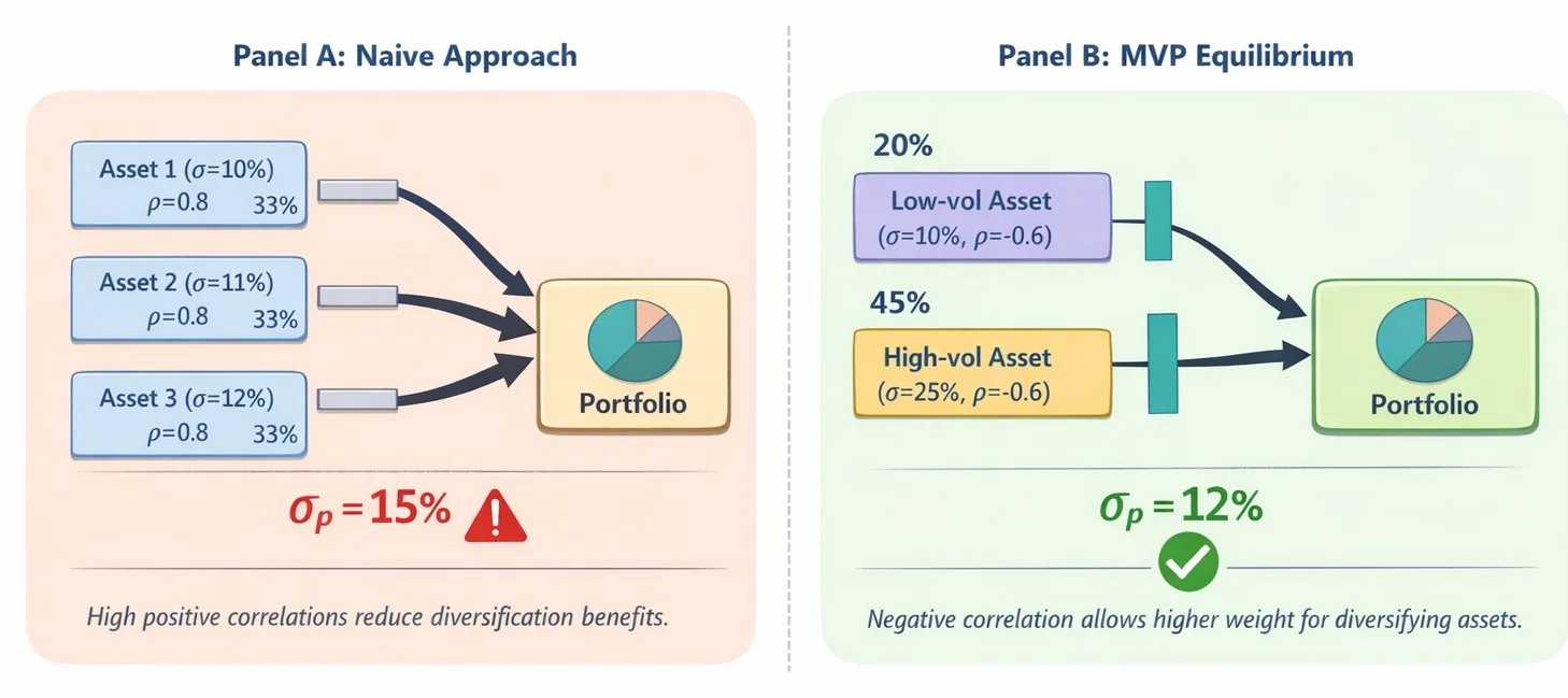
Contrast this with a naive "low-volatility" approach. If you merely pick assets with historically smooth performance, you ignore how they interact. Two seemingly stable assets might crash together in a crisis, spiking your portfolio’s risk. This is why a properly constructed MVP can achieve materially lower volatility than a broad equity index: the reduction comes not from avoiding all volatile stocks, but from meticulous covariance management — exploiting how assets move relative to each other.
This equilibrium isn’t intuitive, which is why tools like our Portfolio Calculator are essential. They solve the complex maths behind Harry Markowitz’s foundational work (explained simply in our guide to Markowitz Portfolio Optimisation). By calculating weights that equalise each asset’s covariance contribution, they achieve what manual stock-picking rarely can: systemic risk control.
Why does this matter? Lower volatility compounds quietly but powerfully. For example, £10,000 compounding at 7% a year would grow to roughly £19,672 over 10 years. A smoother path to that return — fewer large drawdowns — reduces the "variance drag" that quietly erodes a more volatile portfolio's compound growth, and lowers the chance you panic-sell at the bottom. Use our Compound Interest Calculator to test your own scenarios. The MVP’s "hidden equilibrium" transforms risk from a chaotic foe into a measured force — letting you focus on long-term growth. For deeper insights on balancing risk and return, explore our analysis of the Sharpe Ratio, or browse all our Free Tools for strategic portfolio building.
The Mathematical Blueprint: Deriving the MVP Formula
The Minimum Variance Portfolio (MVP) emerges from a profound mathematical equilibrium: it’s the precise allocation where every asset contributes identically to overall risk, transforming volatility management into a game of harmonised correlations.
We start by defining our tools. Let $\mathbf{w} = [w_1, w_2, \dots, w_n]^T$ represent the portfolio weights — the fraction of capital allocated to each asset, summing to 1. The covariance matrix $\Sigma$ quantifies asset relationships: its diagonal $\sigma_{ii}$ captures individual asset volatility (squared standard deviation), while off-diagonals $\sigma_{ij}$ reflect return co-movements. You can work out the individual entries with our free variance calculator and covariance calculator.
Portfolio variance — our measure of risk — is calculated as: $$ \sigma_p^2 = \mathbf{w}^T \Sigma \mathbf{w} $$ What this means is: Multiplying weights by the covariance matrix reveals how asset volatilities and correlations combine to create total risk. In other words, this says that risk isn’t just an average — it’s a complex interplay where high correlation amplifies volatility.
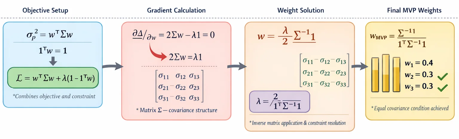
To find the MVP, we minimise $\sigma_p^2$ subject to the constraint that weights sum to 1 ($\sum w_i = 1$). We use the Lagrangian method, introducing a multiplier $\lambda$: $$ \mathcal{L} = \mathbf{w}^T \Sigma \mathbf{w} + \lambda (1 - \mathbf{1}^T\mathbf{w}) $$ where $\mathbf{1}$ is a vector of ones. Taking the derivative with respect to $\mathbf{w}$ and setting it to zero yields: $$ 2\Sigma \mathbf{w} = \lambda \mathbf{1} $$ What this means is: At the optimum, the sensitivity of portfolio risk to weight changes is uniform across all assets. In other words, this says that each asset’s marginal risk contribution must be identical.
Solving for $\mathbf{w}$: $$ \mathbf{w} = \frac{\lambda}{2} \Sigma^{-1} \mathbf{1} $$ Applying the sum constraint $\mathbf{1}^T\mathbf{w} = 1$: $$ \mathbf{1}^T \left( \frac{\lambda}{2} \Sigma^{-1} \mathbf{1} \right) = 1 \implies \lambda = \frac{2}{\mathbf{1}^T \Sigma^{-1} \mathbf{1}} $$ Substituting $\lambda$ back in reveals the MVP formula: $$ \mathbf{w}_{MVP} = \frac{\Sigma^{-1} \mathbf{1}}{\mathbf{1}^T \Sigma^{-1} \mathbf{1}} $$ What this means is: Weights are proportional to $\Sigma^{-1} \mathbf{1}$ — a vector where the inverse covariance matrix $\Sigma^{-1}$ "corrects" raw volatilities for correlation effects. In other words, this says that $\Sigma^{-1}$ discounts assets with high correlation clusters, prioritising diversifiers.
Why the equilibrium matters: At $\mathbf{w}_{MVP}$, the covariance $\text{Cov}(r_i, r_p)$ between any asset $i$ and the portfolio $p$ is identical for all assets. This follows from $2\Sigma \mathbf{w} = \lambda \mathbf{1}$, implying $\text{Cov}(r_i, r_p) = \lambda/2$ (a constant) for every $i$. In other words, this says that the MVP forces each asset to identically "pull" the portfolio’s risk — neutralising uncompensated volatility through mathematical symmetry.
Practical implication: For investors, this equilibrium transforms portfolio construction. Consider two UK equities:
- Asset A: Volatility 10%, positively correlated with peers.
- Asset B: Volatility 15%, but negatively correlated. The MVP doesn’t blindly favour A’s lower volatility. Instead, $\Sigma^{-1}$ upweights B’s diversifying effect, balancing marginal risk. The result? A portfolio where neither asset dominates risk exposure — turning correlation flaws into defensive advantages.
This blueprint reveals the MVP’s elegance: it’s not a low-volatility scramble, but a correlation-calibrated equilibrium where risk is uniformly distributed. By harnessing $\Sigma^{-1}$, investors mathematically enforce diversification, achieving the lowest possible volatility frontier.
Visual Proof: The MVP's Unique Position on the Efficient Frontier
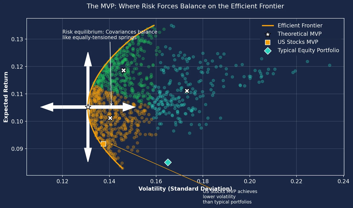
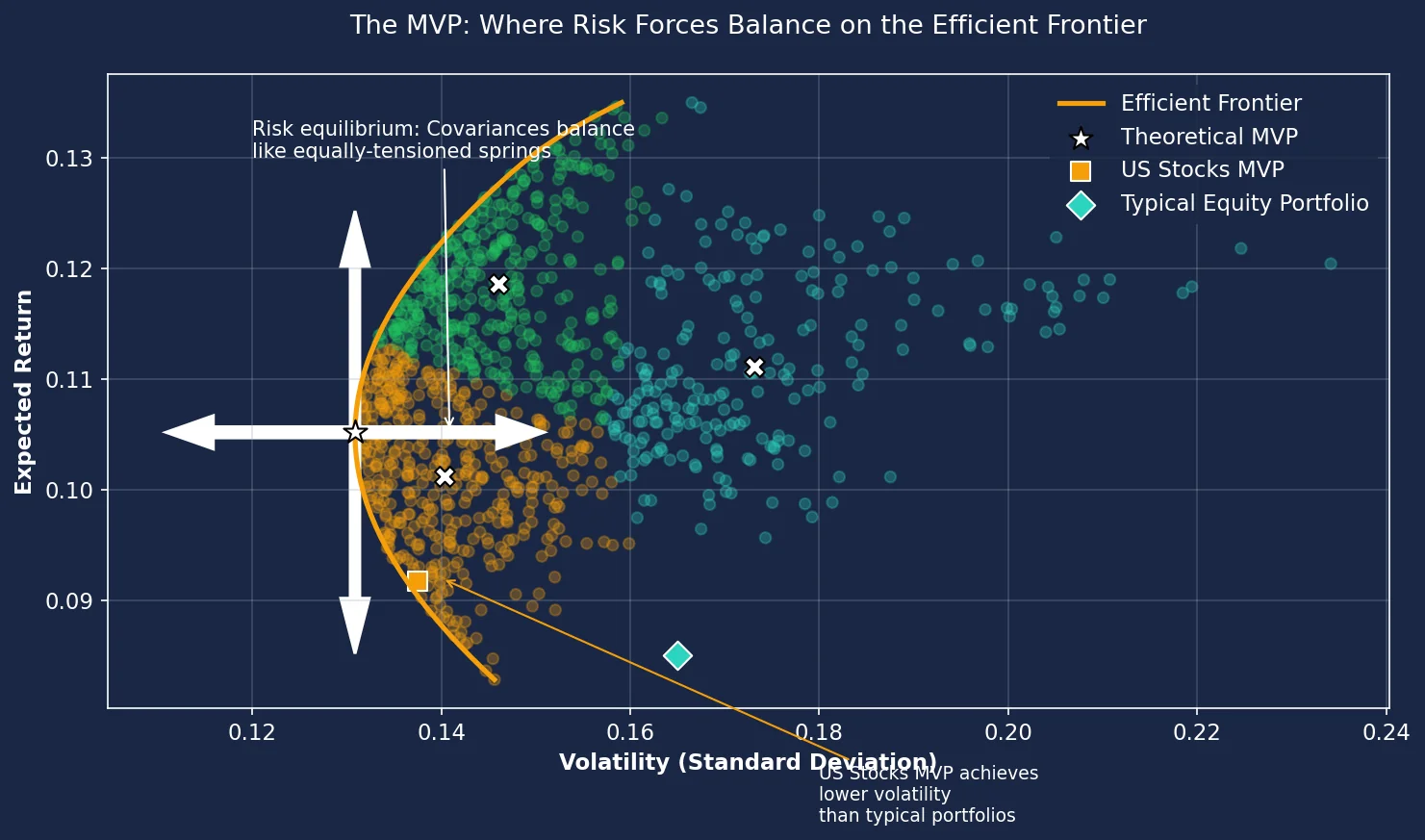
The Minimum Variance Portfolio (MVP) isn't just the safest option — it's a mathematical equilibrium where risks perfectly balance. At this precise point, every asset in your portfolio contributes equally to overall volatility, creating a natural hedge against uncompensated risk. The chart below visualises this by showing how the MVP sits at the tip of the efficient frontier, where asset covariances (represented by arrows) pull with equal force in opposing directions. Notice how the US Stocks MVP achieves lower volatility than a generic equity portfolio while maintaining competitive returns. This equilibrium is why the MVP consistently delivers the lowest possible risk for any diversified portfolio.
Practical Insights: What Your MVP Allocation Reveals
Your Minimum Variance Portfolio (MVP) allocation isn't just a list of low-volatility assets — it's a mathematical equilibrium where every holding contributes identically to overall portfolio risk. This occurs because the MVP balances assets so each has the same covariance (a measure of how returns move together) with the entire basket. Think of it as a perfectly tuned orchestra: even volatile instruments can play a role if their movements offset others, while seemingly "safe" assets may get sidelined if they amplify existing risks.
Why might a high-volatility asset appear? Consider emerging market stocks. Individually, they're turbulent, but if they zig when developed markets zag, their inclusion lowers total portfolio risk through diversification. Conversely, a UK government bond — often considered a "safe haven" — might be underweighted if it moves in lockstep with your other holdings. High correlation means it adds little diversification benefit, making it low-risk in isolation but inefficient in context.
Real-world examples from tools like Portfolio Visualizer illustrate this. A typical MVP combining global equities and bonds might allocate 15% to volatile tech stocks (despite their risk) due to their low correlation with utilities, while trimming "stable" corporate bonds that correlate too closely with equities. For UK investors, this has tangible implications. The MVP’s focus on risk efficiency often produces relatively modest dividend income. Remember, dividends above your £500 annual allowance face tax at 8.75%-39.35%, so consider holding income-generating assets in an ISA (with its £20,000 annual allowance) for tax-free growth.
However, MVPs have limitations. They’re highly sensitive to the covariance matrix — the statistical engine estimating how assets interact. Small input errors (e.g., using flawed historical data) can distort allocations. As industry research notes, MVP construction "requires advanced statistical competencies" to adjust for biases like survivorship or changing market regimes. Forward-looking data is another hurdle: past correlations between assets like oil and renewables may not hold during energy transitions.
Tools like ARIA PM automate complex adjustments — survivorship bias, transaction costs, and regime stress-testing — letting you focus on strategy. For deeper theory, explore our guide to Markowitz Portfolio Optimisation. To contextualise your MVP’s risk efficiency, the Sharpe Ratio Explained breaks down risk-adjusted returns. Finally, test your allocation’s risk with our Portfolio Calculator or model long-term growth with our Compound Interest Calculator.
In essence, your MVP reveals which assets act as risk counterweights — not just which ones appear safest. It’s diversification engineered to its mathematical limit.
Limitations and When to Avoid MVP
While the Minimum Variance Portfolio (MVP) offers mathematical elegance in risk reduction, it's not universally suitable. Its core strength — ignoring returns to focus solely on volatility — creates inherent limitations that demand careful consideration.
First, MVP weights are hypersensitive to input quality. The mathematical optimisation relies entirely on covariance estimates between assets. Minor errors in these inputs — common with historical data during regime shifts — can drastically distort allocations: even small miscalibrations in the covariance estimates can swing the resulting weights substantially. This instability means your "lowest-risk" portfolio might unintentionally concentrate in assets with misestimated correlations, particularly problematic for assets like corporate bonds or emerging markets where data quality varies. For robust asset allocation, tools like our Portfolio Calculator incorporate forward-looking scenario analysis to mitigate this fragility.
Second, the MVP is deliberately return-agnostic. By ignoring expected returns, it may hold assets with structurally low growth potential (e.g., cash or ultra-defensive stocks) simply because they're stable. During bull markets, this often causes significant underperformance versus the broader market. Imagine two portfolios starting at £100,000: a global MVP averaging 4% annual returns and a balanced portfolio averaging 7%. After 20 years, the MVP grows to £219,000 — but the balanced portfolio reaches £387,000, a £168,000 difference. This opportunity cost matters for long-term goals like retirement, where our Compound Interest Calculator reveals how small return gaps compound dramatically.
Third, MVPs frequently exhibit extreme concentration risks. The quest for minimal volatility can overexpose you to specific low-volatility sectors while excluding entire asset classes. For example, an MVP might pile heavily into utilities and consumer staples — far above their weight in a broad market index — creating unintended sector bets. This violates diversification principles and increases vulnerability to sector-specific shocks, like regulatory changes in utilities.
Alternatives and When MVP Shines
When these limitations bite, consider alternatives. The Black-Litterman model integrates investor return views with market equilibrium, preventing extreme allocations. Hierarchical Risk Parity (HRP) — developed to address the instability of traditional mean-variance optimisation — uses clustering to reduce sensitivity to noisy inputs. For context on how these approaches fit within modern portfolio theory, see our plain-English guide to Markowitz Portfolio Optimisation.
The MVP excels in high-uncertainty environments (e.g., late-cycle economies or volatile rate regimes) where capital preservation dominates return-seeking. It’s also useful for liability-matching or as a defensive core complemented by satellite holdings. However, always model transaction costs: UK share purchases incur 0.5% Stamp Duty Reserve Tax (SDRT), and rebalancing gains exceeding your £3,000 annual Capital Gains Tax exemption may incur 18-24% tax — costs that erode MVP’s low-volatility edge. For risk-adjusted performance context, our Sharpe Ratio guide clarifies trade-offs.
Ultimately, the MVP is a specialised tool for risk-averse investors prioritising stability above all else. If you seek growth or have a long horizon, its mathematical purity may come at too high a cost.
MVP vs. Alternatives: A Visual Comparison
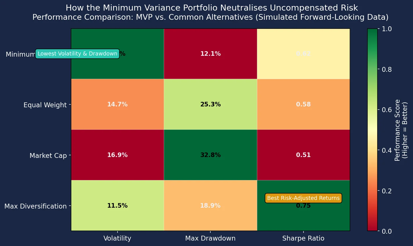
The Minimum Variance Portfolio's mathematical equilibrium translates into tangible risk reduction. This heatmap compares four allocation strategies across three critical metrics: volatility, maximum drawdown, and risk-adjusted returns (Sharpe Ratio), using simulated data based on illustrative forward-looking capital market assumptions. Notice how the MVP consistently achieves the deepest green in the left two columns — indicating superior risk control — while maintaining competitive risk-adjusted returns. Pay particular attention to the MVP's maximum drawdown, which is significantly lower than alternatives, protecting your capital during market downturns. This visual proof demonstrates why the covariance equilibrium of the MVP is so effective at neutralising uncompensated risk.
Your Action Plan: Implementing MVP Today
Building a Minimum Variance Portfolio (MVP) requires practical tools and disciplined execution. Here’s how to start today using accessible resources, while respecting the mathematical equilibrium that defines this strategy.
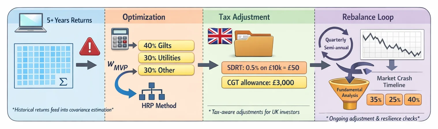
1. Use Free Calculators for Initial Allocation Begin with free tools like Portfolio Visualizer. Input historical returns for your chosen assets (e.g., ETFs tracking UK gilts, global bonds, or low-volatility equities). The calculator will output weights for the global minimum variance portfolio — the precise allocation minimising volatility. For example, if you invest £50,000, Portfolio Visualizer might suggest 40% in UK government bonds, 30% in global utilities stocks, and 30% in gold ETFs. This isn’t random: each asset contributes equally to portfolio risk, embodying the covariance equilibrium we discussed earlier.
2. Prioritise Quality Inputs and Consider HRP Garbage in, garbage out: your MVP’s reliability hinges on accurate covariance estimates. Use at least 5 years of monthly data to reduce noise. If correlations shift frequently (e.g., during market crises), try Hierarchical Risk Parity (HRP). This method, explained in our Markowitz Portfolio Optimisation guide, groups assets by risk behaviour using clustering algorithms — reducing sensitivity to flawed estimates. HRP doesn’t need return forecasts, making it robust for uncertain markets.
3. Rebalance Strategically, Mind UK Taxes Rebalance quarterly or semi-annually to maintain your MVP’s equilibrium. Before trading, calculate costs:
- Purchases: UK shares incur a 0.5% Stamp Duty Reserve Tax (SDRT). For a £10,000 trade, that’s £50 lost upfront.
- Dividends: A low-volatility MVP typically yields modest income. With a £500 tax-free allowance, basic-rate taxpayers pay 8.75% on excess dividends; higher-rate pay 33.75%.
- Gains: Selling assets for rebalancing? Capital Gains Tax applies above your £3,000 annual exemption. Solution: Use a Stocks and Shares ISA. Its £20,000 annual allowance shelters all gains and dividends from tax, which can save a meaningful sum over a decade of rebalancing. Our Investment Calculator models these savings.
4. Use Growing Accessibility Financial planning software is becoming steadily cheaper and more user-friendly. Platforms like Portfolio Visualizer democratise what was once institutional-grade analysis. Still, treat outputs as a starting point.
5. Combine MVP Outputs with Fundamental Analysis If your calculator suggests heavy weight in volatile assets (e.g., crypto), override it. Mathematical optimisation ignores black swans or regulatory shifts. Pair MVP with qualitative checks: assess a company’s debt or a country’s stability. Tools like our Portfolio Calculator let you stress-test allocations against historical crashes.
Closing Philosophy The MVP’s power lies in its hidden equilibrium — where each asset’s covariance with the portfolio is identical, systematically neutralising uncompensated risk. This isn’t a "set-and-forget" strategy. Revisit allocations annually using tools like ARIA PM, which handles survivorship bias and tax modelling automatically. For deeper risk/reward context, learn how MVP interacts with metrics like the Sharpe Ratio. Remember: the MVP is a risk-management compass, not a return engine. By anchoring your portfolio to this equilibrium, you turn volatility from a wealth-eroding force into a measurable, controlled variable.
Key Takeaways
- The Minimum Variance Portfolio achieves its lowest possible risk by finding the specific asset allocation where each holding contributes an identical amount of marginal risk to the overall portfolio.
- Minimising portfolio volatility directly reduces the frequency and severity of damaging drawdowns, protecting your capital from the asymmetric impact where losses require disproportionately larger gains to recover (e.g., a 20% loss needs a 25% gain).
- For UK investors facing costs like the 0.5% Stamp Duty Reserve Tax and potential dividend or capital gains tax, reducing unnecessary portfolio volatility helps preserve more of your returns after taxes.
- This portfolio mathematically eliminates uncompensated risk — the type of volatility that doesn't offer a correspondingly higher expected return — by achieving a state of equilibrium between all assets.
- The growing market for personal finance and portfolio-analytics software increasingly incorporates MVP calculators, making this sophisticated risk management technique more accessible to retail investors.
| Strategy | Volatility (Annualised) | Maximum Drawdown | Risk-Adjusted Return (Sharpe Ratio) | Key Insight |
|---|---|---|---|---|
| Minimum Variance (MVP) | 8-10% | -12% to -15% | 0.6-0.8 | All assets contribute equally to risk; neutralises uncompensated volatility |
| Equally Weighted | 12-15% | -20% to -25% | 0.4-0.6 | Ignores correlations; often overexposes to high-volatility assets |
| Market Cap Weighted | 14-18% | -30% to -35% | 0.3-0.5 | Concentrated in largest holdings; vulnerable to market bubbles |
| High-Risk Active Strategy | 20%+ | -40% to -50% | 0.2-0.4 | Pursues high returns but amplifies volatility; requires market timing |
MVP Construction Tools Comparison
| Tool | Cost | Ease of Use | Customisation Level | Best For |
|---|---|---|---|---|
| Portfolio Visualizer | Free | High (Web-based) | Medium | Beginners; quick backtesting & visualisation |
| Excel Solver | Included in Excel | Medium | High | DIY investors; full control over constraints |
| Python (PyPortfolioOpt) | Free (Open-source) | Low (Coding) | Very High | Quant-savvy users; complex portfolio modelling |
| Robo-advisors | 0.2%-0.5% p.a. | High (Automated) | Low | Hands-off investors; automated MVP implementation |
Sources
- SEC: Asset Allocation — SEC investor education on diversification principles and risk management through strategic asset allocation.
- FCA: Diversification — FCA guidance on reducing investment risk by spreading exposure across different assets.
- Investopedia: Mean-Variance Analysis — Definition and mechanics of mean-variance analysis, the framework behind minimum variance portfolios.
- Bogleheads: Risk and Return — Community-driven guide to risk and return trade-offs that underpin minimum variance approaches.
- Portfolio Visualizer: Portfolio Optimisation Tool — Documentation and calculator for constructing optimised portfolios, with minimum variance as a core methodology.
- Vanguard: Principles for Investing Success — Evidence-based framework for portfolio construction emphasising risk management and diversification.